Pearson's Chi-Square Test with Excel

MS Excel has many built-in statistical features; one of the most useful of which is the chi-square goodness-of-fit test. Although serious statisticians use more sophisticated tools such as SPSS for chi-square and other tests, Excel is easy to use and more ubiquitous, making it easy to share data with others.

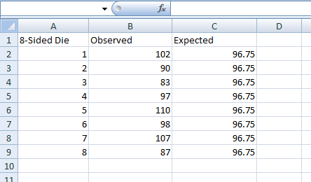
(Step 1) Open a new Excel workbook and label cell A1 with the name of the experiment, cell B1 with the word "Observed," and cell C1 with the word "Expected."

(Step 2) Starting with cell A2 and going down the column, label each category in the experiment. For example, if you are testing the outcomes of rolling an 8-sided die, you could label cells A2 through A9 with the numbers 1 through 8.

(Step 3) Fill out the observed values starting in cell B2, and the expected values starting in cell C2. For example, suppose you roll the 8-sided die 774 times. You would have 8 observations in cells B2 through B9, while cells C2 through C9 would contain the number 96.75, since the expected values of a fair 8-sided die equal 774/8. See image below.



(Step 4) Next, select a cell below the data you entered. In this cell type

=CHITEST(B2:B9;C2:C9)

and hit enter. Excel internally computes the chi-square value and degrees of freedom and outputs the probability. See image below.



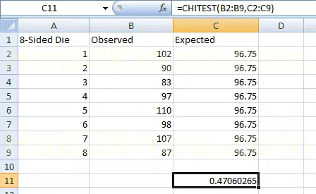
Given the high probability in this experiment, you could conclude that the die is fair and any variations are due to chance.

© Had2Know 2010